After talking about conception and handling of metadata with grid variables in Matillion in the first part of this blog series, we now take a closer look at this issue: How do I use and operationalize these data now?
Step 3: Using metadata
Now let's also have a look at a specific use of the created metadata. It is to be found firstly in the "stage data" step of the "Source2ODS" main job, and secondly in the three transformations "stage2ods_diff", "stage2ods_update" and "stage2ods_insert".
Let's first take a closer look at the staging of the source data.
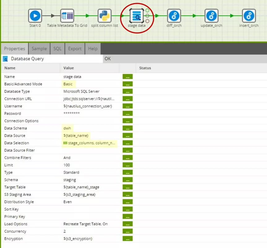
We will use the basic version of the database query component here. This means that the schema and name of the source table as well as the columns to be loaded are selected separately or, as in our use case, set via variables. In the advanced mode, a SELECT statement can also be passed to the component. For us, however, basic mode is completely sufficient here.
In the "data source" parameter, we will again use the "table_name" job variable. In the "data selection" parameter, we use the "column_name" column of the "stage_columns" grid variable. The component therefore reads only the source table's columns which are entered in the "stage_columns" grid variable. Because the "stage_columns" grid variable was derived from the metadata of the "${table_name}_hist" ODS table, only the columns actually needed for the ODS table are read. Columns can now be added and deleted in the source table as required, as long as they do not appear in the ODS table – and, of course, the primary key must remain constant.
The remaining parameters concern the technical connection to the data source, as well as temporary caching of data in an S3 bucket, as required by Matillion and Redshift. However, these parameters are not relevant to the focus of this article. Delta detection makes use of grid variables at various points in the transformation.
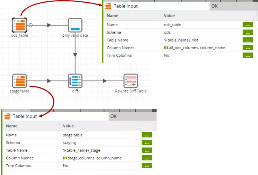
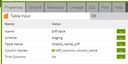
As with the "data source" and "data selection" parameters of the staging step, variables are also used for the table input components. Because the ODS table is slightly wider than the stage table - due to the additional presence of "valid_from" and "valid_to" - different grid variables are used here.
Because the table input component does not offer a direct filtering option, we also need the explicit "only valid data" filter which restricts to currently valid data records ("valid_to" equals '2999-12-31'). Only these data sets are relevant for comparison.
The actual delta step, indeed, makes use of three grid variables.
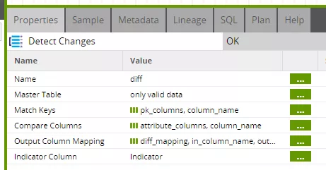
Here we need the lists of key attributes ("pk_columns") and comparison attributes ("attribute_columns"), as well as the mapping of both input tables to the component output ("diff_mapping").
The component performs, as it were, a full outer join between the input tables, and marks the result set with the result of the comparison:
- I identical both data sets are identical
- C changed both data sets are different
- N new the data set is new-
- D deleted the data set has been deleted
Because, in addition to the key attributes and comparison attributes, we also included the "valid_from" column from the ODS table in the mapping, we can use it in the subsequent step to make things much easier for us there.
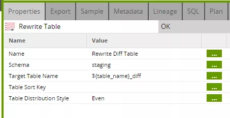
The final "rewrite table" step saves the result of the comparison in an intermediate table. This is recreated (overwritten) during each new process. It consists of all columns of the input data stream, and therefore does not require an explicit column list.
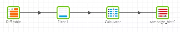
Die Update-Transformation sieht auf den ersten Blick recht einfach aus.
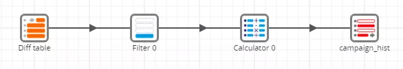
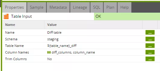
The table input component now refers to the determined delta. The "diff_columns" grid variable is used as the column list. Here, it is interesting to have a closer look at the columns actually contained (see step 2 of the first blog post).
On invocation, the main job only passed "pk_columns" - i.e. the list of key attributes - as "diff_columns" to the update job. The update job then added the "valid_from" and "indicator" columns to this list before passing the variable to the transformation. The remaining columns are not needed to update the "valid_to" date, and therefore do not need to be read from the "diff" table at all.
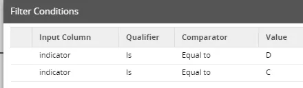
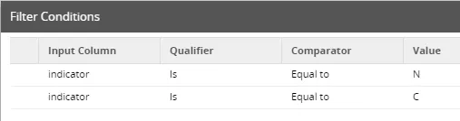
The filter ensures that the "valid_to" date is set only for deleted or changed records.
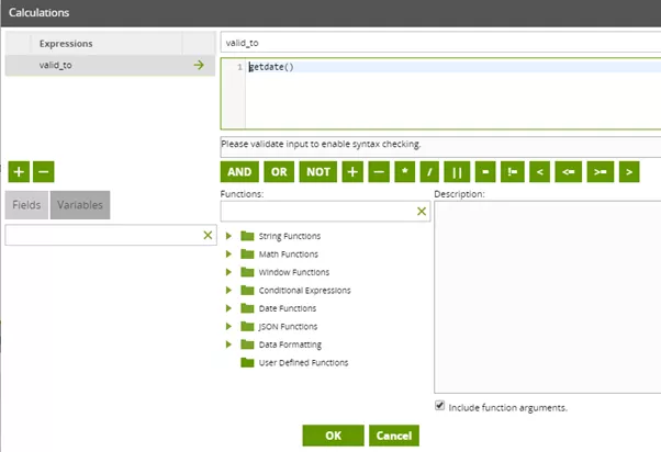
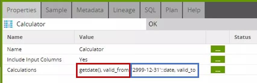
The "calculator" step defines the value to be set for "valid_to". In the example, we do this with the "getdate()" Redshift function which returns the current date in each case.
Remaining finally is the actual update which is again controlled via grid variables.
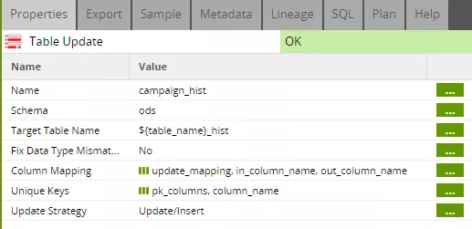
Here we first need a mapping between the component's input columns and the destination table's columns. Because we initially took our column names from the ODS table, which is the update's destination table, the column names are identical in each case. Nevertheless, the component requires explicit mapping, which is created in the update job (see step 2). In addition, the component needs the list of key attributes which we have placed in the "pk_columns" grid variable. The "valid_from" column is now also included here to ensure that only the current version of a data set is found and modified. This addition to the "pk_columns" was also performed in the update job (see step 2).
At first glance, the "insert" transformation looks similar to the "update" transformation.
The "table input" component is, indeed, parameterized completely identically, although the "diff_columns" grid variable here contains the complete column list, except "valid_from".
The filter ensures that only new or changed data sets are entered.
In the "calculator" step, the "getdate()" function is used this time as the value for "valid_from", while "valid_to" is set to the default value '2999-12-31'.
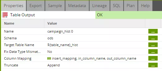
The final "output" component again requires mapping of the column names between the component's input and the destination table. For this, we use the "insert_mapping" grid variable created in the insert job (see step 2).
Step 4: Operationalization
So far, we have only considered the loading process for a single source table. To apply this to an entire source system, we simply need to call the "Source2ODS" main job repeatedly with the different table names. Matillion offers various iterator components for this.
Let's use the grid iterator here. This iterator calls the "Source2ODS" job as many times as rows appear in the grid variable. The values in the grid's individual cells can then be used as transfer parameters during invocation.
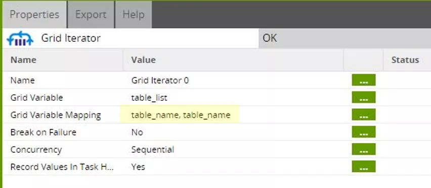
We use the "table_list" grid variable here, and assign the value of the "table_name" column to a scalar "table_name" variable.
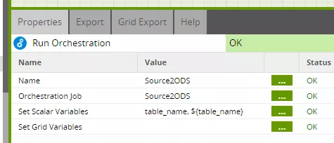
The "table_name" variable is used again as the call parameter for the "Source2ODS" job, and is passed specifically to the "table_name" job variable here.
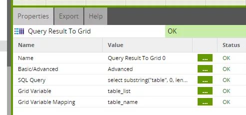
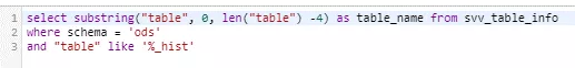
We fill the "table_list" grid variable via a targeted query to the "svv_table_info" metadata view.
This gives us a single job for automatic filling of our operational data store. New columns and even new tables can be easily created in the target schema, and are filled automatically during the next loading – without any change to the ETL process at all.
This brief guide allows you to fully automate technical loading of your DWH and historicization of source data. This leaves plenty of time to take care of the really important tasks in data warehousing – namely to create professional added value for your users!
Do you have any questions about this topic or would like to learn more about Matillion? I look forward to an exchange!