

Do you want to prepare a Power BI report, but the data quantity is too large to even start creating visuals? Or you've actually managed to prepare the report based on such data, but Power BI desktop keeps seizing up? Or the report takes forever to be published? You're not alone here. We will therefore next provide a few tips which are easy to implement.
Tip 1: Separate pbix file as data set
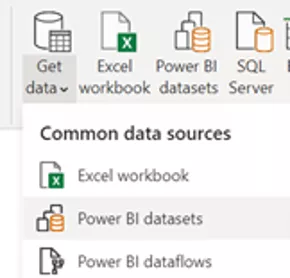
If the amount of data is so large that it takes a long time to upload the desktop file to the Power BI service, we recommend separating the data set from the report file. This means that the data connection is developed as usual in a pbix file, but without creating a report page in it. This is then the data set. It is published inside a workspace to the service, so that any number of further reports (this time only with report pages) can be added.
Separating development of report pages from that of data sets has the following advantages:
- The data set and reports can be edited at the same time.
- The report file becomes smaller and more stable.
- Uploading the report file no longer takes as long.
- Multiple report files can be added on the basis of the same data set, which can be useful for grouping during creation of a Power BI app.
Serving next for further explanation is a simple example of a data warehouse. It is based on an SQL database in Azure. Individual products comprise the smallest component in the Fact_Orders table.

Tip 2: Use of aggregated tables and the composite model
The idea here is as follows: In most cases, the majority of visuals do not at all use the smallest fact component (Product in our example), but aggregate the data (for example, at Customer and OrderDate). Detailed data at the product level are therefore not required at all in such cases. A table with aggregated data suffices instead. Created accordingly is an aggregated fact table which is often much smaller and can therefore be imported.
Still remaining here is the problem with visuals and filters, which still fall back on the product level (for example, for evaluations of sales according to product). In such cases, a fact table at the product level is unavoidable. However, the Direct Query mode is ideal for use with detailed fact tables of this kind.
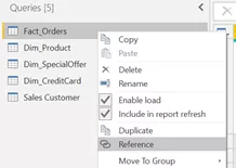
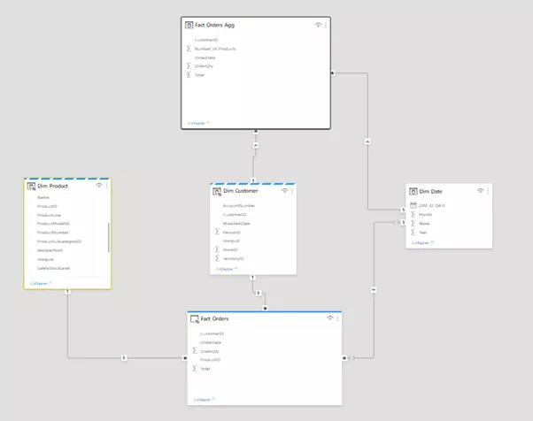
Provided next is a brief guide to practical implementation. In our example, we aggregate the Product dimension, and group it according to the remaining dimensions. First, we create all queries as direct ones in the Power Query editor. The query for the fact table is then referenced and renamed (to Fact_Orders_Agg in this case), and grouping is performed according to the dimensions to be retained (see the diagram).

With the number of rows reduced by aggregation, you can now switch the table in the model view to import mode. Also connected in this process are the dimension tables.
Because the storage mode for each fact table is Direct Query or Import, the storage mode for the dimension tables must be set to Dual. Power BI thus automatically detects which storage mode is optimal for these tables: If data from the aggregated fact table are queried, the data from the dimension tables are used. However, if data at the product level are queried in a visual, for example (via the Fact_Orders table), the data from the Dim_Product table are also fetched via Direct Query.
For this logic to work, however, Power BI needs to be able to differentiate between the aggregation and detail tables.

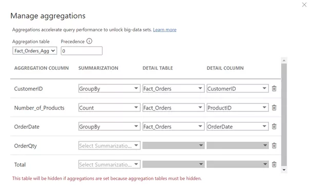
As already evident in the message, the aggregation table is automatically hidden. This means that all visuals appear to be prepared on the basis of the detail table (Fact_Orders), while Power BI retrieves the data according to the logic mentioned above. Here is an example:

The upper diagram contains only data from the aggregation table, so that the saved information is obtained from Power BI. The lower diagram contains a Color field belonging to the Dim_Product table. These data are therefore retrieved via Direct Query.
Tip 3: Parameters for data limitation
Now perhaps even the aggregation table is still relatively large, so that import takes a lot of time. Also large as a result is the file size which occupies the entire main memory and potentially turns publishing into a lengthy process. I therefore recommend the following trick: Create a parameter which limits the number of rows already in the query. This can be realized with a simple if-condition in the extended editor. If you want more homogeneous data for creating visuals, you can add a filter for a calendar week or individual days instead of simply limiting the number of rows.


When you subsequently publish the file, you can set the parameter to 0 in the settings for the data set in the Power BI service. As a result, all data are loaded in the service, while you merely need to handle a subset for development using the desktop version.
Performance issues often occur if large amounts of data are involved. The tips described here are therefore not a conclusive treatment. Rather, there are a wide variety of further optimization options. Information on this is readily available in the Internet or directly in the related Microsoft documentation.