Causality - encounters in everyday life, business intelligence and AI
The topic of causality is being intensely discussed in the machine-learning and data-science communities at present. Only last year in his "Book of Why", Judae Pearl, one of the most famous researchers in the field of Bayesian networks, explained that an understanding of causality will shape the future of artificial intelligence. Also the concept of "prescriptive analytics" as a demarcation or further step after "predictive analytics" is now being discussed everywhere. An understanding of causal relationships is also essential here.

Figure 1: Is the road wet because it is raining or it is raining because the road is wet?
Causality can be found everywhere in our world. As part of very everyday experiences, for example: When it rains, roads become wet. In the business intelligence world too, we can benefit from a better understanding of causal relationships: In order to decide which advertising channel a limited marketing budget is best invested in, we need to understand the impact of the promotional measures as best as possible. In such examples, we can logically argue why one variable depends on another. But what if such information is not available? Or if we simply know nothing at all about the observed variables? This problem is described as causal inference (in the case of two variables):
Two random variables X and Y are in a causal relationship with each other, so that either X —> Y or Y —> X. Based on obervations x, y of the two random variables, is the casual direction X —> Y or Y —> X?

Figure 2: Different causal structures in the two-variable case. Here we are interested only in the two cases above (X —> Y or Y —> X). Special cases are below (no relationship or purely bi-directional relationship).
Causality described statistically with the DO-formalism
The DO-formalism is mostly used to formulate causality in mathematics and statistics. Considered here are conditional probabilities, the condition not being typical observation of a variable P(y|X = x), but intervention in the system and setting of the variable to a value: P(y|do (X = x)). To return to the rain and wet road: In this case there would firstly be a probability of rain if we observed a wet road (very high), as opposed to the probability of rain (no longer as high) if we wet the road with a water hose. This difference tells us something about the causal direction - which is not "wet road" --> "rain", but exactly the reverse.
Examples from the real world
Causal relationships are everywhere; the Tuebingen cause effect pairs are a collection of data records from the real world. Examples here include:
- Elevation and temperature at various locations (the causal direction is height —> temperature)

Figure 3: Height (x-axis) and temperature (y-axis) at various locations
- Drinking-water access and child mortality in different countries
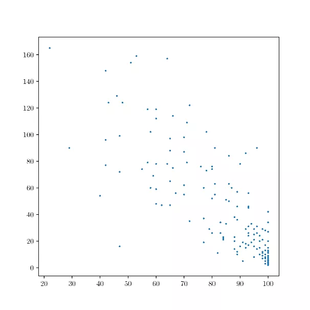
Figure 4: Drinking-water access (x-axis) and child mortality (y-axis) in various countries
- Weight and fuel consumption of different vehicles
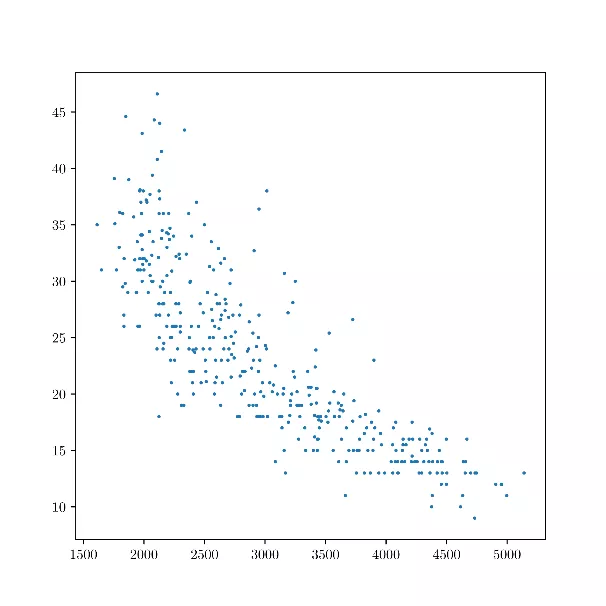
Figure 5: Weight (x-axis) and fuel consumption (y-axis) of different vehicles
The Bayes factor indicates the direction
We are therefore interested in the conditional probabilities for the two models X —> Yand Y —> X, given the data x and y, i.e. P(X —> Y|x,y) and P(Y —> X|x,y). The Bayes factor establishes a relationship between these two probabilities:
![]()
With the Bayes theorem, we can convert this to obtain ![]() . If this factor is larger than 1, then direction X —> Y is more proable; if this factor is smaller than 1, then direction Y —> Xis more proable. To analyze the factors in greater depth, we can also apply the usual conversion for conditional probabilities:
. If this factor is larger than 1, then direction X —> Y is more proable; if this factor is smaller than 1, then direction Y —> Xis more proable. To analyze the factors in greater depth, we can also apply the usual conversion for conditional probabilities:
![]()
Additive noise models
Let us assume that the causal direction is X —> Y. If the causal mechanism is represented by a function f then Y = f(X). This kind of model would still be purely deterministic; we also want to explicitly allow "noise", i.e. a random, stochastic influence E. The additive noise models assume that this noise is added, i.e Y = f(X) + E. As a priori distribution for the causal variable X, the most natural possible distribution function, for example, a Gaussian mixture model, is usually assumed. With it, we can now check a part of the data, namely whether the variable x, which we consider as a cause is really compatible with a priori distribution P(x|X —> Y).
Gaussian process regression
To assess whether observation of the other variable is compatible with a conditional distribution P(y|x, X —> Y) (assuming that y = f (x) + e), we need to consider the function f in more detail. For this, f is treated as a further realization of a random variable. In the framework of Gaussian process regression, f is assumed to be a Gaussian process. In principle, a Gaussian process is a generalization of a random vector with multidimensional, normal distribution towards a continuous function. The covariance matrix of the normal distribution here turns into a continuous covariance operator, typically simply termed kernel. After a particular kernel has been chosen as a hyper parameter (RBF kernels are common here, as also with support vector machines in machine learning, for example), the compatibility of the data with a function f constituting a Gaussian process is considered. GPML for MATLAB is one of the standard libraries; however, Scikit-Learn for Python has also been implemented in the meantime.
Causal generative neural networks
The described methods help us determine the Bayes factor. But there is also a method which employs neural networks. In 2017, causal generative neural networks were presented with the participation of Facebook AI research. This concept makes use of a neural network's ability to universally approximate functions, i.e. basically model any desired function. Here, the network receives observations of a variable such as x,and is trained to use it to subsequently model the other variable, y.Evident in this case too, is an asymmetry between the causal and anti-causal directions. The actual causal direction is typically easier to model than the opposite, anti-causal direction. The direction in which the network can better model the data is then assumed to be the actual direction.
Causal inference in the case of time series - Bayesian structural time series
A use of time series is typical for the initially mentioned example requiring optimal allocation of a marketing budget. The question in this case rather is "what would have happened had things been different", for example, if other channels had been used in past campaigns. This question is typical when one speaks of causal inference in economics; sometimes, one also speaks of Ruben's "Potential Outcome Framework". "Bayesian Structural Time Series" are one of the most modern methods for such analyses. Google has published the CausalImpact library here for the programming language R which makes use of this method. With time-series data collected from past marketing campaigns, we can examine exactly this issue in detail, i.e. assess the turnover which would have been achieved without the corresponding advertising campaigns, for example.
Outlook - causal inference for machine learning
This subject has numerous associations with the world of machine learning. Some of their methods are similar - for example, kernels are also used with the class of the SVM algorithms. Causal generative neural network algorithms are an example of how the ML tool box can be used as an aid in causal inference. However, causal inference can also be understood as part of a larger machine learning scenario. In the case of several variables, causal inference can be used as a first step in an unsupervised learning context to research the causal directions of the variables. Once the variables' causal directions have been determined, work can be performed on specific, predictive models by means of supervised learning.
References:
- Mooij et al.: Distinguishing cause from effect using observational data: methods and benchmarks (JMLR, 2014, https://arxiv.org/abs/1412.3773)
- Mooij et al.: Probabilistic latent variable models for distinguishing between cause and effect (NIPS, 2011)
- Goudet et al.: Causal Generative Neural Networks (arxiv preprint, 2017, https://arxiv.org/abs/1711.08936)