Reinforcement Learning, Bayesian Statistics, and Tensorflow Probability: a child's game - Part 2

In the first part, we explored how Bayesian Statistics might be used to make reinforcement learning less data-hungry. Now we execute this idea in a simple example, using Tensorflow Probability to implement our model.

Rock, paper, scissors

When it comes to games, it is difficult to imagine something simpler than rock, paper, scissors. Despite the simplicity, googling the game reveals a remarkable body of literature. We want to use Bayesian Statistics to play this game and exploit the biases of a human opponent. We will build a model of our opponent’s mind and choose a move which beats it. The most important parts of the code are shown and discussed in this post. If you want to execute the code, use the full notebook. As we want to keep things straightforward, we deal only with the most elementary of biases: We want to model the frequency with which our opponent chooses each of the moves.

Telling a tale of data generation

One of the nice features of the Bayesian approach is that you can come up with a model by just describing the data generating process step by step. Let’s try that for our game:

• Somewhere, deeply hidden in a human mind, there’s a secret probability distribution over the three moves that are possible in this game.
• Governed by this distribution, our human opponent chooses a move.
• This process is repeated over and over, and we count the number of occurrences of rock, paper, and scissors. This is the data we want to use to uncover the secret probability distribution.

Now let’s translate this into a Bayesian model. It is easiest to start with the last step, because it is related to the data we want to use. In this case, the data is simple: It’s just the counts of rock, paper and scissors in the moves of our human opponent from past rounds of the game. When you draw a ball from an urn which contains balls with several colours, put it pack, draw another one, and repeat that, the number of balls you get for each colour is governed by a so-called multinomial distribution.

So, when we say that the counts of each of the three moves are drawn from a multinomial distribution, this is just a fancy way of claiming that they behave like drawing balls from the urn. This also implies that each of the rounds being played is independent of all other rounds. A human player will often employ strategies which lead to dependencies among the rounds, like being hesitant to play the same move more than, say, two or three times in a row. Hence, we already know that independence will not always be perfectly fulfilled. But that doesn’t necessarily mean it’s a bad idea to use it. It could still be a good assumption, if it enables us to play well.

Let’s get Bayesian, baby

Up to this point, there’s nothing specifically Bayesian about our model. Using a multinomial distribution in this context is pretty much a no-brainer for any statistician, even for those who distance themselves passionately from Bayesian approaches.

Genuinely Bayesian is the next step, which requires us to specify which prior knowledge we may want to incorporate into our model regarding the likelihoods of rock, paper and scissors. We do that by specifying a probability distribution that yields combinations of probabilities for rock/ paper/scissors. The so-called Dirichlet distribution is fine for that. If you’ve never heard of the Dirichlet distribution, don’t worry. For our purposes we only need to know that we’re going to use the version that has three parameters, and each of the three parameters will correspond to one of the outcomes of rock/paper/scissors. If one of the parameters (say, the one for paper) is greater than another (e.g., the one for rock), then paper will be more likely than rock under the distribution. If all three parameters are equal to 1, the Dirichlet distribution becomes a uniform distribution. This is the case which we are going to use for the prior. It means that we don’t have any knowledge about which outcome might be more likely than another, and therefore we use a so-called uninformative prior, which doesn’t favour any outcome.

Now our model is ready. It has two steps: In the first one, probabilities for rock, paper and scissors are drawn from a Dirichlet distribution. In the second step, these probabilities are used in a multinomial distribution which generates the counts for each of the moves.

Coding the model

When we translate the ideas from the last paragraph into code, the result looks like this gist.

The first thing you may note is that we’re not calculating a probability here, but the logarithm of a probability. This has purely numerical reasons: The probabilities we work with may be tiny in some cases, tiny enough to cause numerical problems. When we use log probabilities instead, we make better use of the available range of numbers in a floating point value, and numerical problems become much less likely. Working with log probabilities is as simple as working with probabilities directly. You only need to keep in mind that whenever you would multiply probabilities, the corresponding log probabilities must be added.

Now our overall aim in this step is to write a function that returns the joint log probability of a data point (i.e., three counts, one for rock, one for paper, one for scissors) and the corresponding parameter values (here it suffices to have probabilities for rock and paper, the scissors probability can then be calculated). Now the rest is easy: We use the Dirichlet distribution to calculate the log probability of our probability parameter values, the multinomial distribution to calculate the log likelihood of the count values, and then we add the two, which gives us the joint log probability of this data occurring together with these probability parameters (p_rock and p_paper). And that’s it! We’ve coded our Bayesian model.

Estimating parameter values

I just claimed we have a model. But how do you estimate the model’s parameters (specifically, p_rock and p_paper), when all you have is some data and a function for the joint log probability? Fortunately, there is some heavy machinery built into TensorFlow Probability for exactly this job. It’s called Markov chain Monte Carlo, and we’ll use the latest and greatest variant of this method, which goes by the name of Hamilton Monte Carlo. It enables us to sample from the posterior distribution of our model, i.e. the distribution that is derived from the prior by incorporating the information given in the concrete data. And if our sample is large enough, it basically enables us to know everything about that distribution: the shape, the average, the median, the modes, etc. Hamilton Monte Carlo is one of these ideas that sound crazy until you notice how well they work. The intuitive idea is that you imagine the probability you want to sample from as some high-dimensional landscape composed of mountains (high probability) and valleys (low probability). Now you let a ball roll over this surface, and wherever it rolls, it takes samples of the distribution at regular time intervals. But as the ball will gain speed when rolling downhill, it will be much faster in the valleys (and hence, take less samples there) than on the mountains. Surprisingly, this can actually be implemented in a way that works. If you’re interested in more details, read Jeremy Kun’s great introduction to Markov Chain Monte Carlo in general and Richard McElreath’s blog post on Hamilton Monte Carlo in particular. In our case, this piece of code invokes the Hamilton Monte Carlo sampling.

We first define some fictional observed data. In our case, we assume we’ve seen rock five times, but paper and scissor haven’t been chosen yet. Then we do some technical preparation of the Markov Chain and, finally, sample from the chain. When we plot the distribution of samples for p_rock (figure 1, on the left), we see that the median is at 0.8, which is quite reasonable given the fact that the data we threw in is a count of 5 for rock, and zeros for paper and scissors. The plot also shows that there is still substantial uncertainty about the exact value of p_rock. The plots for p_paper and p_scissors (figure 1, in the middle and to the right) show that, as expected, these values are rather close to zero. Now that we’ve estimated the values, we could directly use them for reinforcement learning. But let’s first check that our simulation went right.

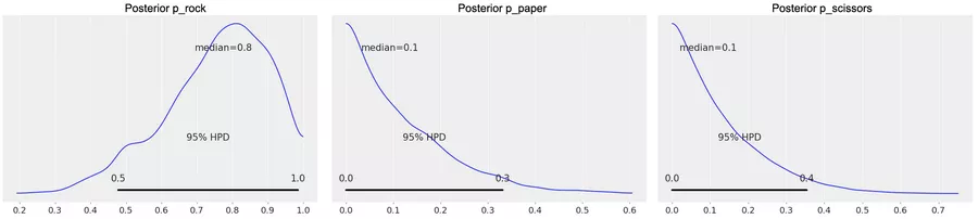
Figure 1

TensorFlow 2 with TensorFlow Probability

If you have tried the Markov chain simulation yourself, you will have noticed that the corresponding cell in the notebook takes about 17 minutes to execute. The reason for this is that it is being executed in eager mode. Tensorflow 2 has execution mechanisms that work similar to the graph mode in TensorFlow 1. However, I could not find out how they can be combined with TensorFlow Probability in order to get a speedup in the Markov chain simulation. As far as I understand, the way we already use “tf.function“ in our code (once as a decorator and once as a function) should do the job. But currently it does not improve the performance. The same code (with slight modifications for graph mode) executes roughly 10x faster in TensorFlow 1. I expect this problem to be solved soon. Maybe someone reading this has an idea, maybe it’s also a matter of waiting for the next version of TensorFlow Probability. Until then, I rather put up with the bad performance than presenting the notebook in Tensorflow 1, which will be legacy soon.

Mathemagically checking our results

Now we’ve used this big black box called Hamilton Monte Carlo for the first time, and it surely would be nice to be able to check that it generates correct results. Fortunately, we are in a very special position: Usually, parameter estimation in Bayesian models needs numerical methods like Hamilton Monte Carlo. But as we kept things very, very simple, we are in one of the very, very few situations in which there is a simple mathematical formula for the parameters. Hence, we have a handy way of double-checking the Monte Carlo results: If we have a Dirichlet prior with parameters (1, 1, 1) and data (r, p, s) (where r/p/s is the number of rock/paper/scissors observations), the corresponding posterior (the distribution we sampled from using Hamilton Monte Carlo) is a Dirichlet(1 + r, 1 + p, 1 + s) distribution. When you compare the corresponding plots of the posterior (figure 2) with the ones we’ve already generated, you’ll notice that they are very similar.

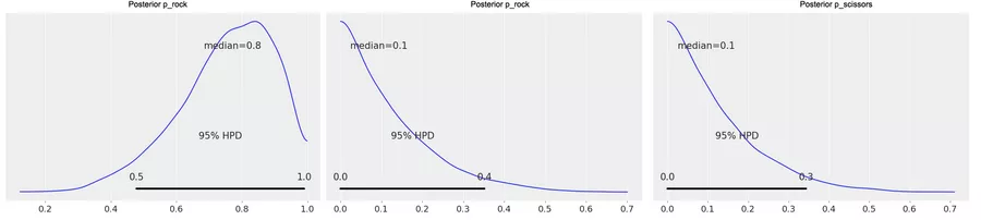
Figure 2

Reinforcement learning: It’s all fun and games

Now it’s time to build our model into a small, reinforcement-learning-powered game of rock, paper, scissors. As the game is more fun when responses are calculated quickly, we will use the mathemagical shortcut from the last paragraph for the calculation of the posterior distribution. This gist contains the main part of the code.

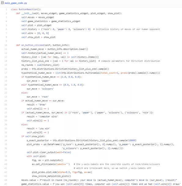
It is being called by the UI code whenever we press one of the buttons in the game. The argument “button_info” is either “rock”, “paper”, or “scissors”. Again, refer to the full notebook if you want to try the game while reading.

The basic idea is that we will use our model to infer the probabilities with which our human opponent chooses each of the moves and update the data and probabilities after each round. Then we draw a likely move of our opponent from this distribution. Calculating our move is then easy: If our opponent chooses rock, we choose paper, if they choose paper, we choose scissors, etc. Hence, we build a randomized strategy that mirrors the actual frequencies with which our opponent chooses each of the moves. The strategy utilizes not only a point estimate, but a full distribution of the likelihoods of each move. You can see how these distributions change during the game. They are shown in a small plot which updates after each move. It is interesting to see how they change, but knowing these distributions gives the human opponent an unfair advantage. You can therefore switch them off by setting “show_plot = False” at the beginning of the cell.

Where do we go from here?

If you’ve made it to this final section, you may (in the best case) have the feeling that all this Bayesian and Markov chain Monte Carlo stuff is intriguing and useful. You may also have the feeling that I skipped over a lot of important detail (which is true). There are some exceptionally well-written books that can fill in the blanks, and I recommend you try one of those. For those who want to approach things from a programming perspective, Cam Davidson-Pilon’s book “Bayesian Methods for Hackers” is a great start. It is available for free on Github, and all the examples have recently been ported to TensorFlow probability. If you’d like to take a slightly more statistics-minded perspective, Richard McElreath’s “Statistical Rethinking” is awesome. The examples are not (yet?) available in TensorFlow Probability. Read the book anyway. Richard McElreath has a marvellous way of demonstrating the simplicity of concepts that sound esoteric when you read about them elsewhere. I should probably recommend some literature on reinforcement learning as well, but I haven’t yet come across a book that I like as much as the ones I just mentioned. I’m curious to hear about your reinforcement learning favourites, and about your adventures when you try all this stuff. Please, feel free to contact me for further discussions!