R is one of the most popular open source programming languages for predictive analytics. One of its upsides is the abundance of modeling choices provided by more than 10000 user-created packages on the Comprehensive R Archive Network (CRAN). On the downside, package-specific syntax choices (which are a much bigger problem in R than in e.g. in Python) impede the employment of new models. The caret package attempts to streamline the process of creating predictive models by providing a uniform interface to various training and prediction functions. Caret’s data preparation- , feature selection- and model tuning functionalities facilitate the process of building and evaluating predictive models. This blog post focuses on model tuning and selection and shows how to tackle common model building challenges with caret.
Between and within-model selection
There is no gold standard: No model beats every other model in every other situation. As data scientists, we have to justify our modelling choices. We select between different models by training them and comparing their performances. The same reasoning applies to parameter choices that are not determined by the optimization process: We select within all models of a class by comparing the performance of models fed by different parameter values.
With caret’s train function we can quickly estimate several different models. As an illustration, we create a predictive model to determine the defaults of credit card holders, based on personal information and their previous payment history.[1]
To select a model we create a small training set, estimate different models for several resamples, compare their performance and deploy the best one.
Data Preprocessing
Caret provides simple functions for creating balanced splits of the data, preserving the overall distribution of the dependent variable. Stratified random sampling is advisable if one class has a disproportionately small frequency compared to others.
library(caret)

set.seed(11)

# reading data and preparation
customer_data <- read.csv("credit_default_prepared.csv", sep = ";",stringsAsFactors = TRUE)

# data partition
rows_train <- createDataPartition(y = customer_data$DEFAULT,
                                  p = 0.3, list = FALSE)
training <- customer_data[rows_train,  ]
A simple but powerful model for binary variables is logistic regression, which we will assess against random forests and boosting. Hence, we will do a between-model selection in which we pit logistic regression against two different ensemble models. Random forests estimate and aggregate several classification trees on bootstrapped subsamples while decorrelating individual trees by means of sampling the set of included predictors. The original boosting algorithm aggregates classification trees too, but estimates them in a sequential fashion:
It starts with equal weights for each observation. In every iteration, the weights of misclassified observations increase and the ones of correctly classified observations decrease. In the next iteration, the updated weights are utilized to concentrate on the correct prediction of previously misclassified observations. The final prediction is obtained by weighting each tree’s prediction based on model accuracy.
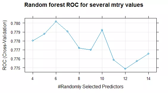
Both ensemble methods include tuning parameters we have to decide upon (within-model selection). For the random forest model, we will only consider the number of predictor variables sampled as candidates at each split (mtry) as a tuning parameter and search through parameter values 4 to 14. Table 1 depicts the tuning parameters for boosting:
Tuningparameter Boosting | Beschreibung | Betrachtete Werte |
Interaction.depth | Number of splits in each tree | 1, 2, 3 |
n.trees | Number of splits in each tree | 80, 100 |
shrinkage | Learning rate, how quickly the weights will adapt | 0,01, 0,1 |
n.minobsinnode | Minimum number of observations in the trees terminal node | 10 |
Expanding the search grid
By default, train uses a minimal search grid of three values for each tuning parameter. With caret’s expand.grid() function we create a Cartesian product of eligible parameters and pass it to the train function:
# parameter grid random forest
grid_rf <- expand.grid(mtry = 4:14)

# parameter grid boosting
grid_bo <- expand.grid(interaction.depth = 1:3,
                    n.trees = seq(80, 100, by = 20),
                    shrinkage = c(0.01, 0.1),
                    n.minobsinnode = 10)
Resampling Techniques and Performance Measures
One approach for model tuning is to fit models with different tuning parameter values to many resampled versions of the training set, estimate their performance and determine the final parameters based on a performance metric.
Choices for the resampling technique and performance measure can be set with the trainControl() function. For this illustration, we do a 5-fold cross-validation and measure model performance by the area under the ROC curve (the default setting in caret is the bootstrap and overall accuracy):
ctrl <- trainControl(
  method = "cv",
  number = 5,
  summaryFunction = twoClassSummary,
  classProbs = TRUE
)
Model Training
The code below shows how to train several different models with caret, substituting only the specific method and the previously specified parameter grid. Caret selects the optimal parameter choice and provides a summary with “print(object_name)”, where “object_name” is the name of the object returned by the train function:
# random forest
set.seed(11)
fit_rf <- train(y ~.,
                data = training,
                method = "rf",
                ntrees = 5,
                metric = "ROC",
                trControl = ctrl,
                tuneGrid = grid_rf)

# boosting
set.seed(11)
fit_bo <- train(y ~.,
                data = training,
                method = "gbm",
                metric = "ROC",
                verbose = FALSE,
                trControl = ctrl,
                tuneGrid = grid_bo)

# performance plot random forest
plot(fit_rf, main = "Random forest ROC for several mtry values")
Plotting the train object displays a performance profile for the tuning parameters. As an example, figure 1 shows the ROC of the random forest in dependence of the number of randomly selected predictors. Choosing six predictors randomly at every split yields to the model with the highest ROC.
Building a good logistic regression model requires great care (i.e. with respect to feature and variable selection). Here we take an arbitrary shortcut by selecting the union of the five most important variables from our boosting and random forest models as predictors. Doing so we introduce caret’s helper function varImp(), which provides us with the ranked importance of the independent variables:
# logistic regression: variable selection
top_n <- function(x, n = 5){
  x <- varImp(x)
  row.names(x$importance)[order(x$importance, decreasing = TRUE)][1:n]
}

lg_par <- unique(as.vector(unique(sapply(list(fit_bo,fit_rf), top_n))))

mt <- model.matrix(~.,data = training)[,lg_par]

# logistic regression
set.seed(11)
fit_lr <- train(mt, training$DEFAULT,
                method = "glm",
                family = binomial,
                metric = "ROC",
                trControl = ctrl)
Model Comparison
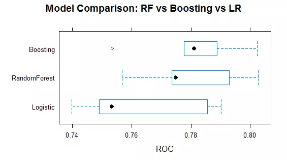
We have just estimated over 120 models and can now visually compare the distribution of their performance. The resamples() function allows to collect, analyse and visualize the resampling results from our data set. Figure 2 summarises the performance distribution for the optimal models over the different folds. Boosting and random forest outperform the ad-hoc logistic regression model. Both ensemble methods perform comparable, but the variance of the boosting algorithm appears to be smaller. For our case study, the average boosting model (ROC: 0.7807) slightly outperforms the average random forest model (ROC of 0.7802).
# Model comparison
comp <- resamples(list(Logistic = fit_lr, RandomForest = fit_rf, Boosting = fit_bo))
summary(comp)

# plot performance comparison
bwplot(comp, metric="ROC", main = "Model Comparison: RF vs Boosting vs LR")
A Cautionary note on utilising caret
The strongest argument for using caret is that it streamlines the model building process, so you can focus on more important modelling decisions: What kind of models could work for your problem at hand? What is the right performance measure? What is the right choice for a parameter space? Caret simplifies model building and selection significantly, but you still need to think:
- Not just choose some models and parameter search spaces to plug into caret’s functions, but the right ones.
- Even more importantly, get the feature engineering right, and tailor it to each of the models you want to use.
[1] The data source is a preprocessed data set from Yeh, I. C., & Lien, C. H. (2009). The comparisons of data mining techniques for the predictive accuracy of probability of default of credit card clients. Expert Systems with Applications, 36(2), 2473-2480ll. (http://archive.ics.uci.edu/ml/datasets/default+of+credit+card+clients). Contact XYC for the prepared version of the data se


